Parameter Sensitivities with OpenModelica¶

This section describes the use of OpenModelica to compute parameter sensitivities using forward sensitivity analysis together with the Sundials/IDA solver.

Single Parameter sensitivities with IDA/Sundials¶

Background¶

Parameter sensitivity analysis aims at analyzing the behavior of the corresponding model states w.r.t. model parameters.

Formally, consider a Modelica model as a DAE system:

$F(x, \dot x, y, p, t) = 0 \; x(t_0) = x_0(p)$

where $x(t) \in \mathbf{R}^n$ represent state variables, $\dot x(t) \in \mathbf{R}^n$ represent state derivatives, $y(t) \in \mathbf{R}^k$ represent algebraic variables, $p \in \mathbf{R}^m$ model parameters.

For parameter sensitivity analysis the derivatives

$\frac{\partial x}{ \partial p}$

are required which quantify, according to their mathematical definition, the impact of parameters $p$ on states $x$ . In the Sundials/IDA implementation the derivatives are used to evolve the solution over the time by:

$\dot s_i = \frac{\partial x}{ \partial p_i}$

An Example¶

This section demonstrates the usage of the sensitivities analysis in OpenModelica on an example. This module is enabled by the following OpenModelica compiler flag:

>>> setCommandLineOptions("--calculateSensitivities")
true

Listing 8 LotkaVolterra.mo¶

model LotkaVolterra
  Real x(start=5, fixed=true),y(start=3, fixed=true);
  parameter Real mu1=5,mu2=2;
  parameter Real lambda1=3,lambda2=1;
equation
  0 = x*(mu1-lambda1*y) - der(x);
  0 = -y* (mu2 -lambda2*x) - der(y);
end LotkaVolterra;

Also for the simulation it is needed to set IDA as solver integration method and add a further simulation flag -idaSensitivity to calculate the parameter sensitivities during the normal simulation.

>>> simulate(LotkaVolterra, method="ida", simflags="-idaSensitivity")
record SimulationResult
    resultFile = "«DOCHOME»/LotkaVolterra_res.mat",
    simulationOptions = "startTime = 0.0, stopTime = 1.0, numberOfIntervals = 500, tolerance = 1e-6, method = 'ida', fileNamePrefix = 'LotkaVolterra', options = '', outputFormat = 'mat', variableFilter = '.*', cflags = '', simflags = '-idaSensitivity'",
    messages = "LOG_SUCCESS       | info    | The initialization finished successfully without homotopy method.
LOG_SUCCESS       | info    | The simulation finished successfully.
",
    timeFrontend = 0.011579385000000001,
    timeBackend = 0.005734688,
    timeSimCode = 0.001599579,
    timeTemplates = 0.004263196,
    timeCompile = 0.732048009,
    timeSimulation = 0.017234565,
    timeTotal = 0.772632395
end SimulationResult;

Now all calculated sensitivities are stored into the results mat file under the $Sensitivities block, where all currently every top-level parameter of the Real type is used to calculate the sensitivities w.r.t. every state.

_images/LotkaVolterraSensitivities.svg — Figure 92 Results of the sensitivities calculated by IDA solver.¶

_images/LotkaVolterraResults.svg — Figure 93 Results of the LotkaVolterra equations.¶

Single and Multi-parameter sensitivities with OMSens¶

OMSens is an OpenModelica sensitivity analysis and optimization module.

Installation¶

The core files of OMSens are provided as part of the OpenModelica installation. However, you still need to install python and build OMSens with that python before using it. Follow the build/install instructions described on the OMSens github page.

Usage¶

OMSens offers 3 flavors for parameter sensitivity analysis.

Individual Sensitivity Analysis

Used to analyze how a parameter affects a variable when perturbed on its own

Multi-parameter Sweep

Exploratory experimentation that sweeps the space of a set of parameters

Vectorial Sensitivity Analysis

Used to find the combination of parameters that maximizes/minimizes a state variable

As an example, we choose the Lotka-Volterra model that consists of a second-order nonlinear set of ordinary differential equations. The system models the relationship between the populations of predators and preys in a closed ecosystem.

model LotkaVolterra "This is the typical equation-oriented model"
  parameter Real alpha=0.1 "Reproduction rate of prey";
  parameter Real beta=0.02 "Mortality rate of predator per prey";
  parameter Real gamma=0.4 "Mortality rate of predator";
  parameter Real delta=0.02 "Reproduction rate of predator per prey";
  parameter Real prey_pop_init=10 "Initial prey population";
  parameter Real pred_pop_init=10 "Initial predator population";
  Real prey_pop(start=prey_pop_init) "Prey population";
  Real pred_pop(start=pred_pop_init) "Predator population";
initial equation
  prey_pop = prey_pop_init;
  pred_pop = pred_pop_init;
equation
  der(prey_pop) = prey_pop*(alpha-beta*pred_pop);
  der(pred_pop) = pred_pop*(delta*prey_pop-gamma);
end LotkaVolterra;

Let's say we need to investigate the influence of model parameters on the predator population at 40 units of time. We assume a +/-5% uncertainty on model parameters.

We can use OMSens to study the sensitivity model to each parameter, one at a time.

Open the Lotka-Volterra model using OMEdit.

Individual Sensitivity Analysis¶

Select Sensitivity Optimization > Run Sensitivity Analysis and Optimization from the menu. A window like the one below should appear. Windows users should use the default python executable that comes with OpenModelica installation i.e., they don't need to change the proposed python executable path. If you want to use some other python installation then make sure that all the python dependencies are installed for that python installation.

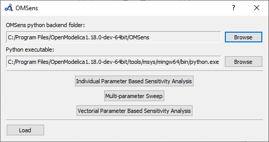
_images/omsens-window.png — Figure 94 OMSens window.¶

Choose Individual Parameter Based Sensitivity Analysis and set up the simulation settings.

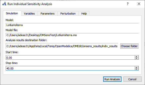
_images/omsens-individual-analysis.png — Figure 95 Run individual sensitivity analysis.¶

Select variables.

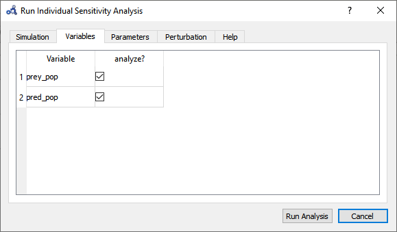
_images/omsens-individual-analysis-variables.png — Figure 96 Individual sensitivity analysis variables.¶

Select parameters.

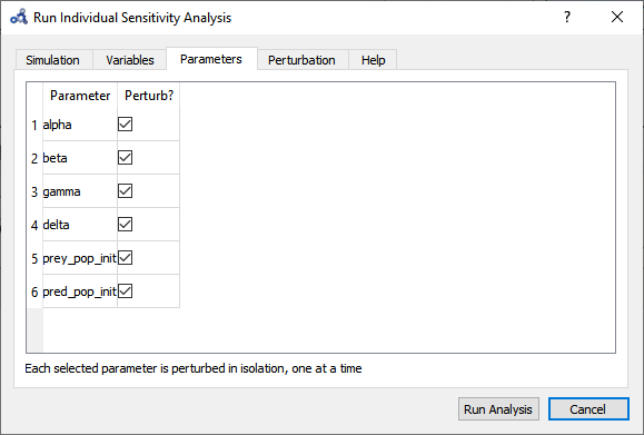
_images/omsens-individual-analysis-parameters.png — Figure 97 Individual sensitivity analysis parameters.¶

Choose the perturbation percentage and direction. Run the analysis.

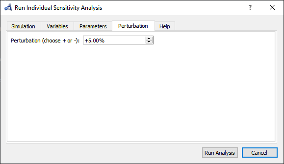
_images/omsens-individual-analysis-perturbation.png — Figure 98 Individual sensitivity analysis perturbation.¶

After the analysis a dialog with results is shown. Open the heatmap corresponding to the relative sensitivity index.

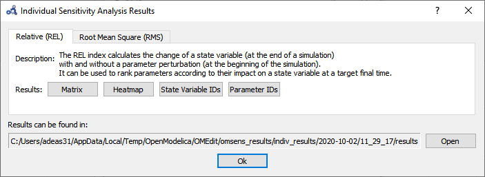
_images/omsens-individual-analysis-results.png — Figure 99 Individual sensitivity analysis results.¶

The heatmap shows the effect of each parameter on each variable in the form of (parameter,variable) cells. As we can see, pred_pop was affected by the perturbation on every parameter but prey_pop presents a negligible sensitivity to delta (P.3). Recall that this heatmap shows the effect on the variables at time 40 for each perturbation imposed at time 0.

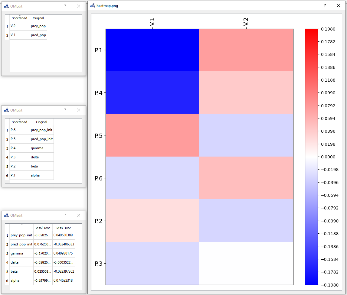
_images/omsens-individual-analysis-heatmap.png — Figure 100 Individual sensitivity analysis heatmap.¶

Multi-parameter Sweep¶

Now we would like to see what happens to pred_pop when the top 3 most influencing parameters are perturbed at the same time. Repeat the first three steps from Individual Sensitivity Analysis but this time select Multi-parameter Sweep.

Choose to sweep alpha, gamma and pred_pop_init in a range of ±5% from its default value and with 3 iterations (#iter) distributed equidistantly within that range. Run the sweep analysis.

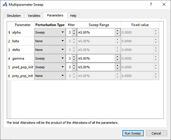
_images/omsens-multi-sweep-parameters.png — Figure 101 Multi-parameter sweep parameters.¶

The backend is invoked and when it completes the analysis the following results dialog is shown. Open the plot for pred_pop.

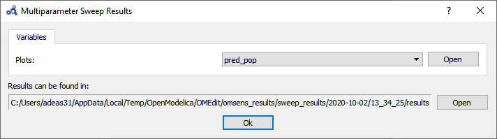
_images/omsens-multi-sweep-results.png — Figure 102 Multi-parameter sweep results.¶

At time 40 the parameters perturbations with a higher predator population are all blue, but it's not clear which one. We need something more precise.

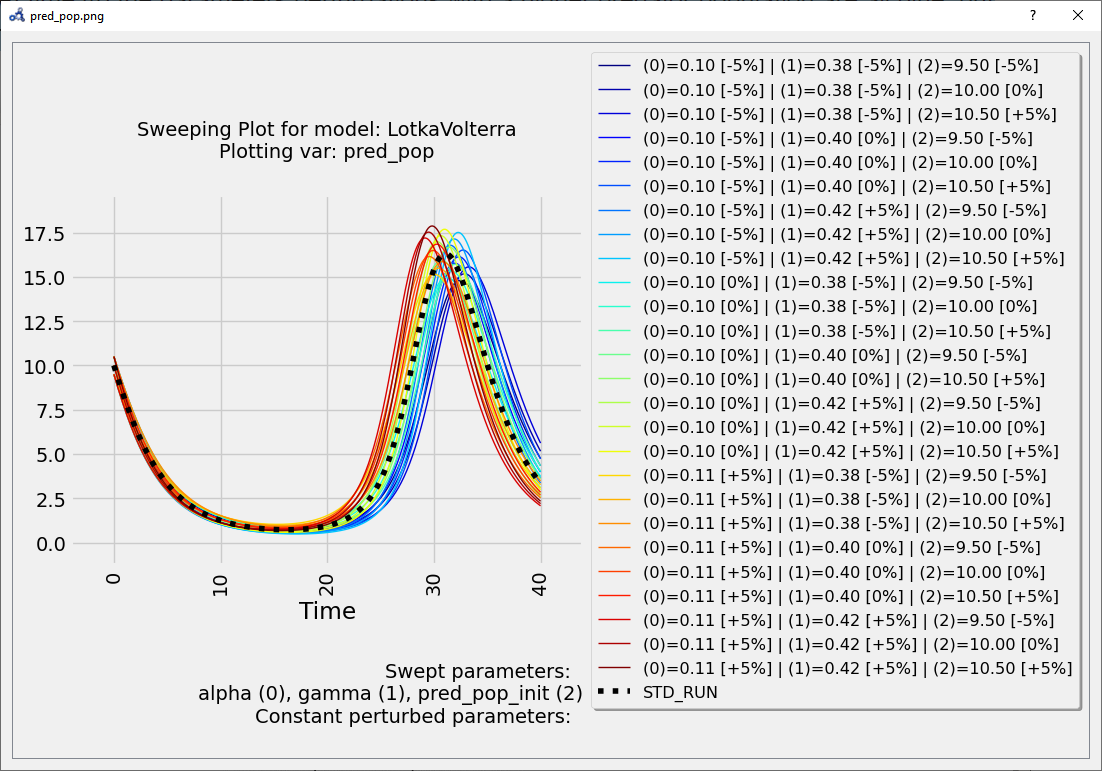
_images/omsens-multi-sweep-plot.png — Figure 103 Multi-parameter sweep plot.¶

These results can be very informative but clearly the exhaustive exploration approach doesn't scale for more parameters (#p) and more perturbation values (#v) (#v^#p simulations required).

Vectorial Sensitivity Analysis¶

Using the Vectorial optimization-based analysis (see below) we can request OMSens to find a combination of parameters that perturbs the most (i.e. minimize or maximize) the value of the target variable at a desired simulation time.

For Vectorial Sensitivity Analysis repeat the first two steps from Individual Sensitivity Analysis but choose Vectorial Parameter Based Sensitivity Analysis.

Choose only alpha, delta and pred_pop_init to perturb.

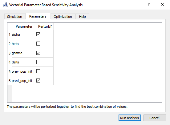
_images/omsens-vectorial-analysis-parameters.png — Figure 104 Vectorial sensitivity analysis parameters.¶

Setup the optimization settings and run the analysis.

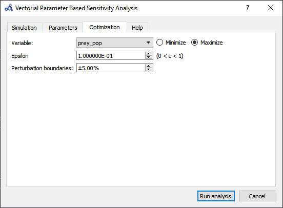
_images/omsens-vectorial-analysis-optimization.png — Figure 105 Vectorial sensitivity analysis optimization.¶

The Parameters tab in the results window shows the values found by the optimization routine that maximize pred_pop at t=40 s.

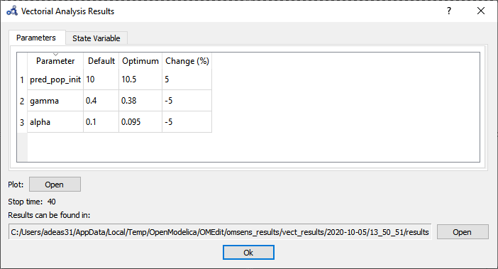
_images/omsens-vectorial-analysis-results.png — Figure 106 Vectorial sensitivity analysis parameters result.¶

The State Variable tab shows the comparison between the values of the variable in the standard run vs the perturbed run at simulation time 40s.

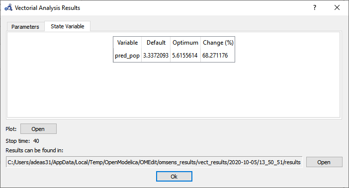
_images/omsens-vectorial-analysis-state-variables.png — Figure 107 Vectorial sensitivity analysis state variables.¶

If we simulate using the optimum values and compare it to the standard (unperturbed) run, we see that it delays the bell described by the variable.

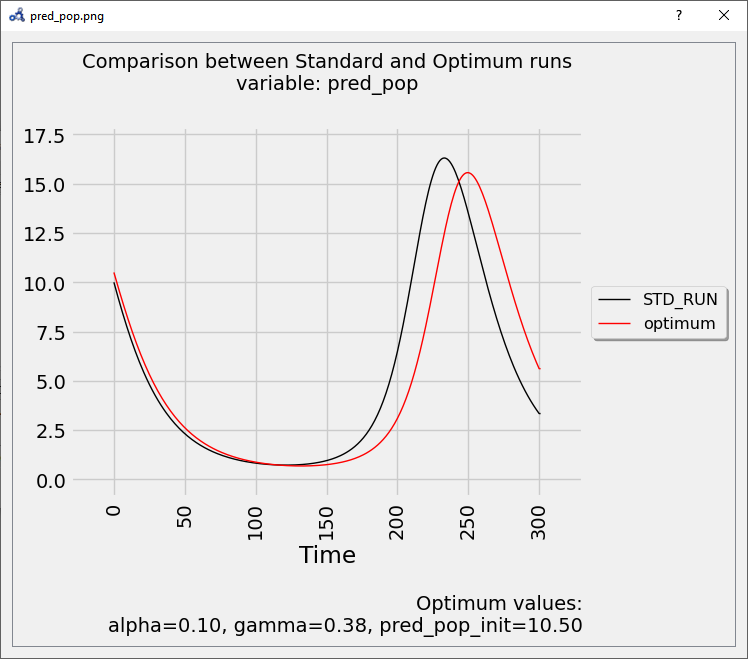
_images/omsens-vectorial-analysis-plot.png — Figure 108 Vectorial sensitivity analysis plot.¶

So far, we have only perturbed the top 3 parameters detected by the Individual Sensitivity method. Maybe we can find a greater effect on the variable if we perturb all 6 parameters. Running a Sweep is not an option as perturbing 6 parameters with 3 iterations each results in 3⁶=729 simulations. We run another Vectorial Sensitivity Analysis instead but now choose to perturb all 6 parameters.

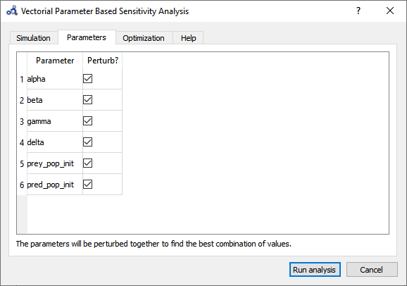
_images/omsens-vectorial-analysis-parameters-all.png — Figure 109 Vectorial sensitivity analysis parameters.¶

The parameters tab shows that the optimum value is found by perturbing all of the parameters to their boundaries.

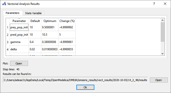
_images/omsens-vectorial-analysis-results-all.png — Figure 110 Vectorial sensitivity analysis parameters result.¶

The State Variable tab shows that pred_pop can be increased by 98% when perturbing the 6 parameters as opposed to 68% when perturbing the top 3 influencing parameters.

The plot shows again that the parameters found delay the bell-shaped curve, but with a stronger impact than before.

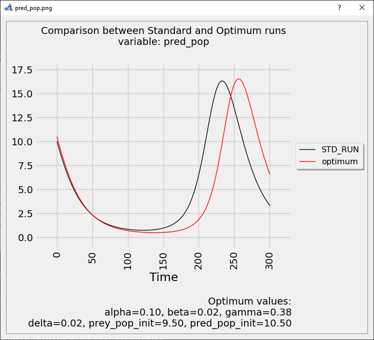
_images/omsens-vectorial-analysis-plot-all.png — Figure 112 Vectorial sensitivity analysis plot.¶