FMI and TLM-Based Simulation and Co-simulation of External Models

Functional Mock-up Interface - FMI

The Functional Mock-up Interface (FMI) Standard for model exchange and co-simulation allows export, exchange and import of pre-compiled models between different tools. The FMI standard is Modelica independent, so import and export works both between different Modelica or non-Modelica tools.

See also OMSimulator documentation.

FMI Export

To export a FMU use the OpenModelica command buildModelFMU() from the command line interface, OMShell, OMNotebook or MDT. The FMU export command is also integrated in OMEdit. Select File > Export > FMU. Or alternatively, right click a model to obtain the export command. The FMU package is generated in the current working directory of OMC or the directory set in OMEdit > Options > FMI > Move FMU. You can use the cd() command to see the current location. The location of the generated FMU is printed in the Messages Browser of OMEdit or on the command line.

You can set which version of FMI to export through OMEdit settings, see section FMI Options.

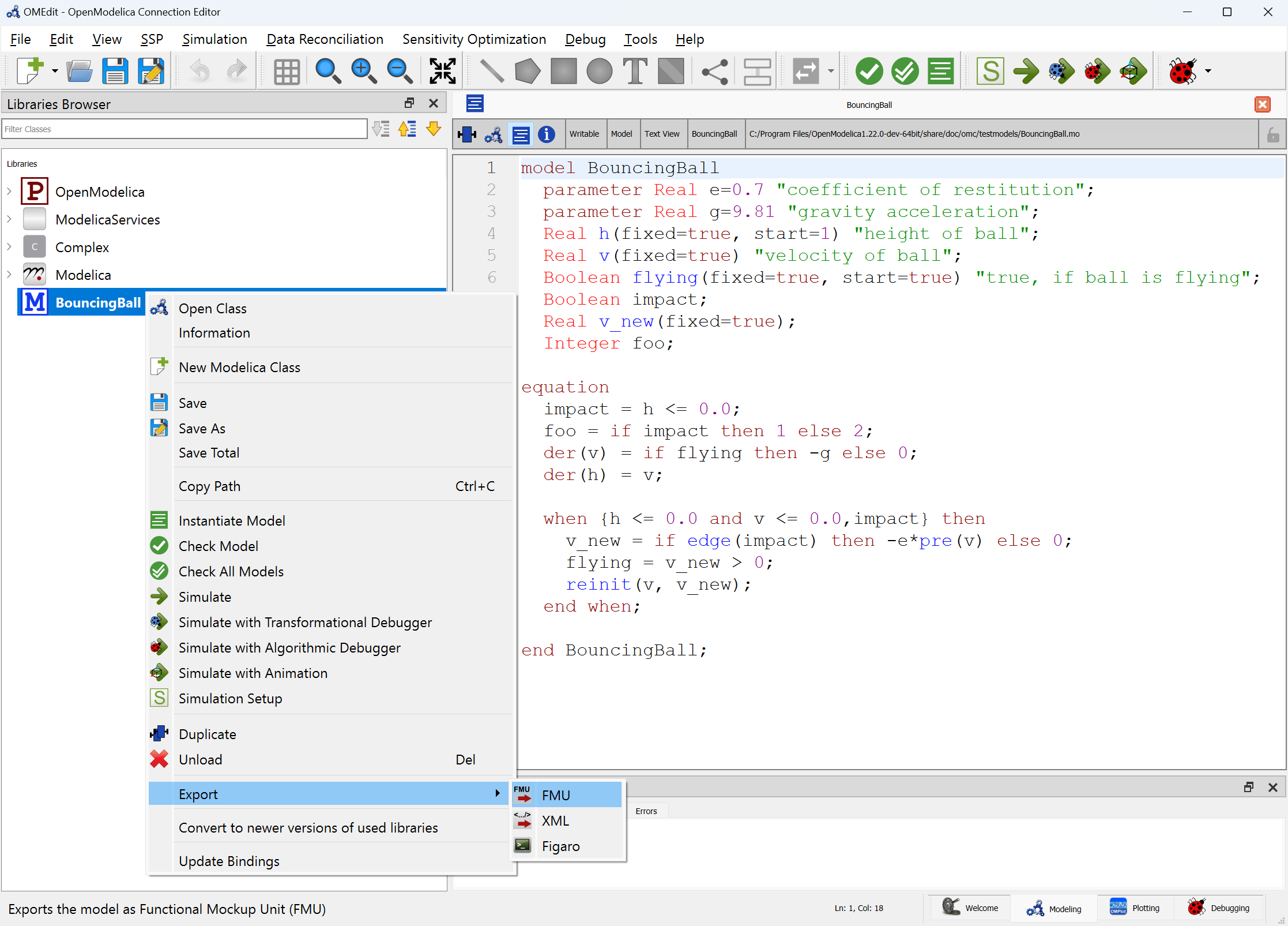
Figure 41 FMI Export.

To export the bouncing ball example to an FMU, use the following commands:

>>> loadFile(getInstallationDirectoryPath() + "/share/doc/omc/testmodels/BouncingBall.mo")
true
>>> buildModelFMU(BouncingBall)
"«DOCHOME»/BouncingBall.fmu"

Note

Notification: Model statistics after passing the front-end and creating the data structures used by the back-end:

* Number of equations: 6

* Number of variables: 6

Notification: Model statistics after passing the back-end for initialization:

* Number of independent subsystems: 3

* Number of states: 0 ()

* Number of discrete variables: 9 (v_new,$PRE.v_new,flying,$PRE.flying,foo,impact,$whenCondition1,$whenCondition2,$whenCondition3)

* Number of discrete states: 0 ()

* Number of clocked states: 0 ()

* Top-level inputs: 0

Notification: Strong component statistics for initialization (13):

* Single equations (assignments): 13

* Array equations: 0

* Algorithm blocks: 0

* Record equations: 0

* When equations: 0

* If-equations: 0

* Equation systems (not torn): 0

* Torn equation systems: 0

* Mixed (continuous/discrete) equation systems: 0

Notification: Model statistics after passing the back-end for simulation:

* Number of independent subsystems: 1

* Number of states: 2 (h,v)

* Number of discrete variables: 7 ($whenCondition3,$whenCondition2,$whenCondition1,flying,impact,v_new,foo)

* Number of discrete states: 2 (impact,v)

* Number of clocked states: 0 ()

* Top-level inputs: 0

Notification: Strong component statistics for simulation (9):

* Single equations (assignments): 7

* Array equations: 0

* Algorithm blocks: 0

* Record equations: 0

* When equations: 2

* If-equations: 0

* Equation systems (not torn): 0

* Torn equation systems: 0

* Mixed (continuous/discrete) equation systems: 0

After the command execution is complete you will see that a file BouncingBall.fmu has been created. Its contents varies depending on the target platform. On the machine generating this documentation the contents in Listing 2 are generated (along with the C source code).

Listing 2 BouncingBall FMU contents

binaries/
binaries/linux64/
binaries/linux64/BouncingBall.so
modelDescription.xml

A log file for FMU creation is also generated named ModelName_FMU.log. If there are some errors while creating the FMU, they will be shown in the command line window and logged in this log file as well.

By default an FMU that can be used for both Model Exchange and Co-Simulation is generated. We support FMI 1.0 & FMI 2.0.4 for Model Exchange FMUs and FMI 2.0.4 for Co-Simulation FMUs.

For the Co-Simulation FMU two integrator methods are available:

• Forward Euler [default]

• SUNDIALS CVODE (see [1])

Forward Euler uses root finding, which does an Euler step of communicationStepSize in fmi2DoStep. Events are checked for before and after the call to fmi2GetDerivatives.

If CVODE is chosen as integrator the FMU should also include runtime dependencies (--fmuRuntimeDepends=modelica) to copy all used dynamic libraries into the generated FMU to make it exchangeable.

To export a Co-Simulation FMU with CVODE for the bouncing ball example use the following commands:

>>> loadFile(getInstallationDirectoryPath() + "/share/doc/omc/testmodels/BouncingBall.mo")
true
>>> setCommandLineOptions("--fmiFlags=s:cvode")
true
>>> buildModelFMU(BouncingBall, version = "2.0", fmuType="cs")
"«DOCHOME»/BouncingBall.fmu"

Note

Notification: Model statistics after passing the front-end and creating the data structures used by the back-end:

* Number of equations: 6

* Number of variables: 6

Notification: Model statistics after passing the back-end for initialization:

* Number of independent subsystems: 3

* Number of states: 0 ()

* Number of discrete variables: 9 (v_new,$PRE.v_new,flying,$PRE.flying,foo,impact,$whenCondition1,$whenCondition2,$whenCondition3)

* Number of discrete states: 0 ()

* Number of clocked states: 0 ()

* Top-level inputs: 0

Notification: Strong component statistics for initialization (13):

* Single equations (assignments): 13

* Array equations: 0

* Algorithm blocks: 0

* Record equations: 0

* When equations: 0

* If-equations: 0

* Equation systems (not torn): 0

* Torn equation systems: 0

* Mixed (continuous/discrete) equation systems: 0

Notification: Model statistics after passing the back-end for simulation:

* Number of independent subsystems: 1

* Number of states: 2 (h,v)

* Number of discrete variables: 7 ($whenCondition3,$whenCondition2,$whenCondition1,flying,impact,v_new,foo)

* Number of discrete states: 2 (impact,v)

* Number of clocked states: 0 ()

* Top-level inputs: 0

Notification: Strong component statistics for simulation (9):

* Single equations (assignments): 7

* Array equations: 0

* Algorithm blocks: 0

* Record equations: 0

* When equations: 2

* If-equations: 0

* Equation systems (not torn): 0

* Torn equation systems: 0

* Mixed (continuous/discrete) equation systems: 0

The FMU BouncingBall.fmu will have a new file BouncingBall_flags.json in its resources directory. By manually changing its content users can change the solver method without recompiling the FMU.

The BouncingBall_flags.json for this example is displayed in Listing 3.

Listing 3 BouncingBall FMI flags

{
  "s" : "cvode"
}

Compilation Process

OpenModelica can export FMUs that are compiled with CMake (default) or Makefiles. CMake version v3.21 or newer is recommended, minimum CMake version is v3.5.

The Makefile FMU export will be removed in a future version of OpenModelica. Set compiler flag --fmuCMakeBuild=false to use the Makefiles export.

The FMU contains a CMakeLists.txt file in the sources directory that can be used to re-compile the FMU for a different host and is also used to cross-compile for different platforms.

The CMake compilation accepts the following settings:

• BUILD_SHARED_LIBS: Boolean value to switch between dynamic and statically linked binaries.

  • ON (default): Compile DLL/Shared Object binary object.

  • OFF: Compile static binary object.

• FMI_INTERFACE_HEADER_FILES_DIRECTORY: String value specifying path to FMI header files containing fmi2Functions.h, fmi2FunctionTypes.h and fmi2TypesPlatforms.h.

  • Defaults to a location inside the OpenModelica installation directory, which was used to create the FMU. They need to be version 2.0.4 from the FMI Standard.

• RUNTIME_DEPENDENCIES_LEVEL: String value to specify runtime dependencies set.

  • none: Adds no runtime dependencies to FMU. The FMU can't be used on a system if it doesn't provided all needed dependencies.

  • modelica (default): Add Modelica runtime dependencies to FMU, e.g. a external C library used from a Modelica function. Needs CMake version v3.21 or newer.

  • all: Add system and Modelica runtime dependencies. Needs CMake version v3.21 or newer.

• NEED_CVODE: Boolean value to integrate CVODE integrator into CoSimulation FMU.

  • ON: Link to SUNDIALS CVODE. If CVODE is not in a default location CVODE_DIRECTORY needs to be set. Its also recommended to use RUNTIME_DEPENDENCIES_LEVEL=modelica or higher to add SUNDIALS runtime dependencies into the FMU.

  • OFF (default): Don't link to SUNDIALS CVODE.

• CVODE_DIRECTORY: String value with location of libraries sundials_cvode and sundials_nvecserial with SUNDIALS version 5.4.0.

  • Defaults to a location inside the OpenModelica installation directory, which was used to create the FMU.

Then use CMake to configure, build and install the FMU. To repack the FMU after installation use custom target create_fmu.

For example to re-compile the FMU with cmake and runtime dependencies use:

$ unzip BouncingBall.fmu -d BouncingBall_FMU
$ cd BouncingBall_FMU/sources
$ cmake -S . -B build_cmake \
  -D RUNTIME_DEPENDENCIES_LEVEL=modelica \
  -D CMAKE_C_COMPILER=clang -D CMAKE_CXX_COMPILER=clang++
$ cmake --build build_cmake --target create_fmu --parallel

Platforms

The platforms setting specifies for what target system the FMU is compiled:

• Empty: Create a Source-Code-only FMU.

• native: Create a FMU compiled for the exporting system.

• <cpu>-<vendor>-<os> host triple: OpenModelica searches for programs in PATH matching pattern <cpu>-<vendor>-<os>cc to compile. E.g. x86_64-linux-gnu for a 64 bit Linux OS or i686-w64-mingw32 for a 32 bit Windows OS using MINGW.

• <cpu>-<vendor>-<os> docker run <image> Host triple with Docker image: OpenModelica will use the specified Docker image to cross-compile for given host triple. Because privilege escalation is very easy to achieve with Docker OMEdit adds --pull=never to the Docker calls for the multiarch/crossbuild images. Only use this option if you understand the security risks associated with Docker images from unknown sources. E.g. x86_64-linux-gnu docker run --pull=never multiarch/crossbuild to cross-compile for a 64 bit Linux OS. Because system libraries can be different for different versions of the same operating system, it is advised to use --fmuRuntimeDepends=all.

FMI Import - SSP

If you want to simulate a single, stand-alone FMU, or possibly a connection of several FMUs, the recommended tool to do that is OMSimulator, see the OMSimulator documentation and Graphical Modelling for further information.

FMI Import - Non-Standard Modelica Model

FMI Import allows to use an FMU, generated according to the FMI for Model Exchange 2.0 standard, as a component in a Modelica model. This can be useful if the FMU describes the behavior of a component or sub-system in a structured Modelica model, which is not easily turned into a pure FMI-based model that can be handled by OMSimulator.

FMI is a computational description of a dynamic model, while a Modelica model is a declarative description; this means that not all conceivable FMUs can be successfully imported as Modelica models. Also, the current implementation of FMU import in OpenModelica is still somewhat experimental and not guaranteed to work in all cases. However, if the FMU-ME you want to import was exported from a Modelica model and only represents continuous time dynamic behavior, it should work without problems when imported as a Modelica block.

Please also note that the current implementation of FMI Import in OpenModelica is based on a built-in wrapper that uses a reinit() statement in an algorithm section. This is not allowed by the Modelica Language Specification, so it is necessary to set the compiler to accept this non-standard construct by setting the --allowNonStandardModelica=reinitInAlgorithms compiler flag. In OMEdit, you can set this option by activating the Enable FMU Import checkbox in the Tools | Options | Simulation | Translation Flags tab. This will generate a warning during compilation, as there is no guarantee that the imported model using this feature can be ported to other Modelica tools; if you want to use a model that contains imported FMUs in another Modelica tool, you should rely on the other tool's import feature to generate the Modelica blocks corresponding to the FMUs.

After setting the --allowNonStandardModelica flag, to import the FMU package use the OpenModelica command importFMU,

>>> list(OpenModelica.Scripting.importFMU, interfaceOnly=true);

The command could be used from command line interface, OMShell, OMNotebook or MDT. The importFMU command is also integrated with OMEdit through the File > Import > FMU dialog: the FMU package is extracted in the directory specified by workdir, or in the current directory of omc if not specified, see Tools > Open Working Directory.

The imported FMU is then loaded in the Libraries Browser and can be used as any other regular Modelica block.

Transmission Line Modeling (TLM) Based Co-Simulation

This chapter gives a short description how to get started using the TLM-Based co-simulation accessible via OMEdit.

The TLM Based co-simulation provides the following general functionalities:

• Import and add External non-Modelica models such as Matlab/SimuLink, Adams, and BEAST models

• Import and add External Modelica models e.g. from tools such as Dymola or Wolfram SystemModeler, etc.

• Specify startup methods and interfaces of the external model

• Build the composite models by connecting the external models

• Set the co-simulation parameters in the composite model

• Simulate the composite models using TLM based co-simulation

Composite Model Editing of External Models

The graphical composite model editor is an extension and specialization of the OpenModelica connection editor OMEdit. A composite model is composed of several external sub-models including the interconnections between these sub-models. External models are models which need not be in Modelica, they can be FMUs, or models accessed by proxies for co-simulation and connected by TLM-connections. The standard way to store a composite model is in an XML format. The XML schema standard is accessible from tlmModelDescription.xsd. Currently composite models can only be used for TLM based co-simulation of external models.

Loading a Composite Model for Co-Simulation

To load the composite model, select File > Open Composite Model(s) from the menu and select compositemodel.xml.

OMEdit loads the composite model and show it in the Libraries Browser. Double-clicking the composite model in the Libraries Browser will display the composite model as shown below in Figure 42.

Figure 42 Composite Model with 3D View.

Co-Simulating the Composite Model

There are two ways to start co-simulation:

• Click TLM Co-Simulation setup button () from the toolbar (requires a composite model to be active in ModelWidget)

• Right click the composite model in the Libraries Browser and choose TLM Co-Simulation setup from the popup menu (see Figure 43)

Figure 43 Co-simulating and Fetching Interface Data of a composite model from the Popup Menu .

The TLM Co-Simulation setup appears as shown below in Figure 44.

Figure 44 TLM Co-simulation Setup.

Click Simulate from the Co-simulation setup to confirm the co-simulation. Figure 45 will appears in which you will be able to see the progress information of the running co-simulation.

Figure 45 TLM Co-Simulation Progress.

The editor also provides the means of reading the log files generated by the simulation manager and monitor. When the simulation ends, click Open Manager Log File or Open Monitor Log File from the co-simulation progress bar to check the log files.

Plotting the Simulation Results

When the co-simulation of the composite model is completed successful, simulation results are collected and visualized in the OMEdit plotting perspective as shown in Figure 46 and Figure 47. The Variables Browser display variables that can be plotted. Each variable has a checkbox, checking it will plot the variable.

Figure 46 TLM Co-Simulation Results Plotting.

Figure 47 TLM Co-Simulation Visualization.

Preparing External Models

First step in co-simulation Modeling is to prepare the different external simulation models with TLM interfaces. Each external model belongs to a specific simulation tool, such as MATLAB/Simulink*, BEAST, MSC/ADAMS, Dymola and Wolfram SystemModeler.

When the external models have all been prepared, the next step is to load external models in OMEdit by selecting the File > Load External Model(s) from the menu.

OMEdit loads the external model and show it in the Libraries Browser as shown below in Figure 48.

Figure 48 External Models in OMEdit.

Creating a New Composite Model

We will use the "Double pendulum" composite model which is a multibody system that consists of three sub-models: Two OpenModelica Shaft sub-models (Shaft1 and Shaft2) and one SKF/BEAST bearing sub-model that together build a double pendulum. The SKF/BEAST bearing sub-model is a simplified model with only three balls to speed up the simulation. Shaft1 is connected with a spherical joint to the world coordinate system. The end of Shaft1 is connected via a TLM interface to the outer ring of the BEAST bearing model. The inner ring of the bearing model is connected via another TLM interface to Shaft2. Together they build the double pendulum with two shafts, one spherical OpenModelica joint, and one BEAST bearing.

To create a new composite model select File > New Composite Model from the menu.

Your new composite model will appear in the in the Libraries Browser once created. To facilitate the process of textual composite modeling and to provide users with a starting point, the Text View (see Figure 49) includes the composite model XML elements and the default simulation parameters.

Figure 49 New composite model text view.

Adding Submodels

It is possible to build the double pendulum by drag-and-drop of each simulation model component (sub-model) from the Libraries Browser to the Diagram View. To place a component in the Diagram View of the double pendulum model, drag each external sub-model of the double pendulum (i.e. Shaft1, Shaft2, and BEAST bearing sub-model) from the Libraries Browser to the Diagram View.

Figure 50 Adding sub-models to the double pendulum composite model.

Fetching Submodels Interface Data

To retrieve list of TLM interface data for sub-models, do any of the following methods:

• Click Fetch Interface Data button () from the toolbar (requires a composite model to be active in ModelWidget)

• Right click the composite model in the Library Browser and choose Fetch Interface Data from the popup menu (see Figure 43).

To retrieve list of TLM interface data for a specific sub-model,

• Right click the sub-model inside the composite model and choose Fetch Interface Data from the popup menu.

Figure 51 will appear in which you will be able to see the progress information of fetching the interface data.

Figure 51 Fetching Interface Data Progress.

Once the TLM interface data of the sub-models are retrieved, the interface points will appear in the diagram view as shown below in Figure 52.

Figure 52 Fetching Interface Data.

Connecting Submodels

When the sub-models and interface points have all been placed in the Diagram View, similar to Figure 52, the next step is to connect the sub-models. Sub-models are connected using the Connection Line Button () from the toolbar.

To connect two sub-models, select the Connection Line Button and place the mouse cursor over an interface and click the left mouse button, then drag the cursor to the other sub-model interface, and click the left mouse button again. A connection dialog box as shown below in Figure 53 will appear in which you will be able to specify the connection attributes.

Figure 53 Sub-models Connection Dialog.

Continue to connect all sub-models until the composite model Diagram View looks like the one in Figure 54 below.

Figure 54 Connecting sub-models of the Double Pendulum Composite Model.

Changing Parameter Values of Submodels

To change a parameter value of a sub-model, do any of the following methods:

• Double-click on the sub-model you want to change its parameter

• Right click on the sub-model and choose Attributes from the popup menu

The parameter dialog of that sub-model appears as shown below in Figure 55 in which you will be able to specify the sub-models attributes.

Figure 55 Changing Parameter Values of Sub-models Dialog.

Changing Parameter Values of Connections

To change a parameter value of a connection, do any of the following methods:

• Double-click on the connection you want to change its parameter

• Right click on the connection and choose Attributes from the popup menu.

The parameter dialog of that connection appears (see Figure 53) in which you will be able to specify the connections attributes.

Changing Co-Simulation Parameters

To change the co-simulation parameters, do any of the following methods:

• Click Simulation Parameters button () from the toolbar (requires a composite model to be active in ModelWidget)

• Right click an empty location in the Diagram View of the composite model and choose Simulation Parameters from the popup menu (see Figure 56)

Figure 56 Changing Co-Simulation Parameters from the Popup Menu.

The co-simulation parameter dialog of the composite model appears as shown below in Figure 57 in which you will be able to specify the simulation parameters.

Figure 57 Changing Co-Simulation Parameters Dialog.

Footnotes

[1]

Sundials Webpage