Modelica Performance Analyzer

A common problem when simulating models in an equation-based language like Modelica is that the model may contain non-linear equation systems. These are solved in each time-step by extrapolating an initial guess and running a non-linear system solver. If the simulation takes too long to simulate, it is useful to run the performance analysis tool. The tool has around 5~25% overhead, which is very low compared to instruction-level profilers (30x-100x overhead). Due to being based on a single simulation run, the report may contain spikes in the charts.

When running a simulation for performance analysis, execution times of user-defined functions as well as linear, non-linear and mixed equation systems are recorded.

To start a simulation in this mode, turn on profiling with the following command line flag >>> setCommandLineOptions("--profiling=all")

The generated report is in HTML format (with images in the SVG format), stored in a file modelname_prof.html, but the XML database and measured times that generated the report and graphs are also available if you want to customize the report for comparison with other tools.

Below we use the performance profiler on the simple model A:

model ProfilingTest
  function f
    input Real r;
    output Real o = sin(r);
  end f;
  String s = "abc";
  Real x = f(x) "This is x";
  Real y(start=1);
  Real z1 = cos(z2);
  Real z2 = sin(z1);
equation
  der(y) = time;
end ProfilingTest;

We simulate as usual, after setting the profiling flag:

>>> setCommandLineOptions("--profiling=blocks+html")
true
>>> simulate(ProfilingTest)
record SimulationResult
    resultFile = "«DOCHOME»/ProfilingTest_res.mat",
    simulationOptions = "startTime = 0.0, stopTime = 1.0, numberOfIntervals = 500, tolerance = 1e-6, method = 'dassl', fileNamePrefix = 'ProfilingTest', options = '', outputFormat = 'mat', variableFilter = '.*', cflags = '', simflags = ''",
    messages = "LOG_SUCCESS       | info    | The initialization finished successfully without homotopy method.
LOG_SUCCESS       | info    | The simulation finished successfully.
Warning: empty y range [3:3], adjusting to [2.97:3.03]
Warning: empty y range [3:3], adjusting to [2.97:3.03]
Warning: empty y range [2:2], adjusting to [1.98:2.02]
Warning: empty y range [2:2], adjusting to [1.98:2.02]
Warning: empty y range [3:3], adjusting to [2.97:3.03]
Warning: empty y range [3:3], adjusting to [2.97:3.03]
LOG_STDOUT        | info    | Time measurements are stored in ProfilingTest_prof.html (human-readable) and ProfilingTest_prof.xml (for XSL transforms or more details)
",
    timeFrontend = 0.001943786,
    timeBackend = 0.007446768,
    timeSimCode = 0.0010759180000000001,
    timeTemplates = 0.002553469,
    timeCompile = 0.290540039,
    timeSimulation = 0.032813406,
    timeTotal = 0.336448016
end SimulationResult;
"Warning: There are nonlinear iteration variables with default zero start attribute found in NLSJac0. For more information set -d=initialization. In OMEdit Tools->Options->Simulation->Show additional information from the initialization process, in OMNotebook call setCommandLineOptions(\"-d=initialization\").
Warning: The initial conditions are not fully specified. For more information set -d=initialization. In OMEdit Tools->Options->Simulation->Show additional information from the initialization process, in OMNotebook call setCommandLineOptions(\"-d=initialization\").
"

Profiling information for ProfilingTest

Information

All times are measured using a real-time wall clock. This means context switching produces bad worst-case execution times (max times) for blocks. If you want better results, use a CPU-time clock or run the command using real-time priviliges (avoiding context switches).

Note that for blocks where the individual execution time is close to the accuracy of the real-time clock, the maximum measured time may deviate a lot from the average.

For more details, see ProfilingTest_prof.xml.

Settings

Name	Value
Integration method	dassl
Output format	mat
Output name	ProfilingTest_res.mat
Output size	24.0 kB
Profiling data	ProfilingTest_prof.data
Profiling size	0 B

Summary

Task	Time	Fraction
Pre-Initialization	0.000119	5.44%
Initialization	0.000129	5.89%
Event-handling	0.000000	0.00%
Creating output file	0.000149	6.81%
Linearization		NaN%
Time steps	0.001413	64.55%
Overhead	0.000141	6.44%
Unknown	NaN	NaN%
Total simulation time	0.002189	100.00%

Global Steps

	Steps	Total Time	F raction	Average Time	Max Time	De viation
|Graph th umbnail 999|	499	0 .001413	64.55%	2.8316 6332665 331e-06	0.00 0060654	20.42x

Measured Function Calls

	Name	Calls	Time	F raction	Max Time	De viation
|Graph th umbnail f unction fun0| |Graph th umbnail count f unction fun0|	` Profili ngTest. f <#lin e=0>`__	1512	0.00 0030500	1.39%	0.00 0000371	17.39x

Measured Blocks

	Name	Calls	Time	F raction	Max Time	De viation
|Graph th umbnail eq0| |Graph th umbnail count eq0|	` <# eq0>`__	8	0.00 0070127	3.20%	0.00 0070271	7.02x
|Graph th umbnail eq11| |Graph th umbnail count eq11|	` <#e q11>`__	4	0.00 0002042	0.09%	0.00 0002104	3.12x
|Graph th umbnail eq19| |Graph th umbnail count eq19|	` <#e q19>`__	1006	0.00 0485104	22.16%	0.00 0022903	46.50x
|Graph th umbnail eq21| |Graph th umbnail count eq21|	` <#e q21>`__	1508	0.00 0511504	23.37%	0.00 0021441	62.21x

Equations

Name	Variables
eq0
eq1	y
eq2	s
eq3	z1
eq4
eq5	` <#var0>`__
eq6	` <#var0>`__
eq7	` <#var0>`__
eq8	` <#var0>`__
eq9	z2
eq10
eq11	x
eq12
eq13	z2
eq14
eq15	` <#var0>`__
eq16	` <#var0>`__
eq17	` <#var0>`__
eq18	` <#var0>`__
eq19	z1
eq20
eq21	x
eq22	der(y)
eq23

Variables

Name	Comment
y
der(y)
x	This is x
z1
z2
s

---

This report was generated by OpenModelica on 2024-04-26 16:18:01.

Genenerated JSON for the Example

Listing 9 ProfilingTest_prof.json

{
"name":"ProfilingTest",
"prefix":"ProfilingTest",
"date":"2024-04-26 16:18:01",
"method":"dassl",
"outputFormat":"mat",
"outputFilename":"ProfilingTest_res.mat",
"outputFilesize":24581,
"overheadTime":0.00014542,
"preinitTime":0.000119354,
"initTime":0.000128641,
"eventTime":0,
"outputTime":0.000148924,
"jacobianTime":6.00227e-06,
"totalTime":0.00218942,
"totalStepsTime":2.61452e-06,
"totalTimeProfileBlocks":0.00106878,
"numStep":499,
"maxTime":6.0653515e-05,
"functions":[
{"name":"ProfilingTest.f","ncall":1512,"time":0.000030500,"maxTime":0.000000371}
],
"profileBlocks":[
{"id":0,"ncall":8,"time":0.000070127,"maxTime":0.000070271},
{"id":11,"ncall":4,"time":0.000002042,"maxTime":0.000002104},
{"id":19,"ncall":1006,"time":0.000485104,"maxTime":0.000022903},
{"id":21,"ncall":1508,"time":0.000511504,"maxTime":0.000021441}
]
}

Using the Profiler from OMEdit

When running a simulation from OMEdit, it is possible to enable profiling information, which can be combined with the transformations browser.

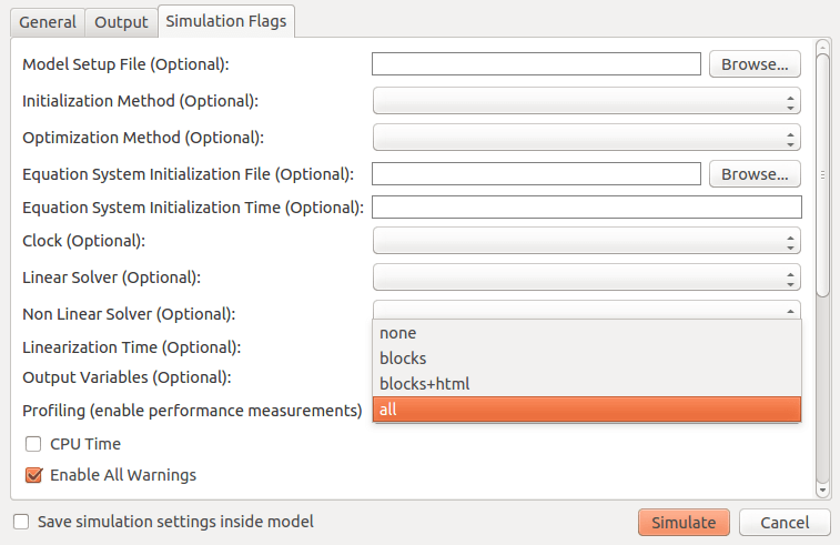
Figure 136 Setting up the profiler from OMEdit.

When profiling the DoublePendulum example from MSL, the following output in Figure 137 is a typical result. This information clearly shows which system takes longest to simulate (a linear system, where most of the time overhead probably comes from initializing LAPACK over and over).

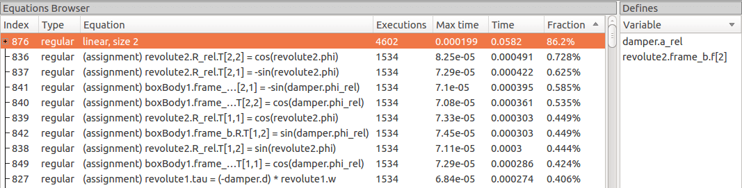
Figure 137 Profiling results of the Modelica standard library DoublePendulum example, sorted by execution time.